![]()
In this part Real Time Stocks Prediction Using Keras LSTM Model, we will write a code to understand how Keras LSTM Model is used to predict stocks. We have used TESLA STOCK data-set which is available free of cost on yahoo finance. Please download data-set from here. On the other way there will be different dependencies which will also be downloaded to run this code. We are listing these as below.
Requirements for running the code for Keras LSTM Model:
- Python 2/3. Please download python by visiting here.
- Pandas for data analysis. Once python is downloaded you can install pandas with the help of pip. Please type this in terminal
pip/pip3 install pandas
- Matplotlib to see the prediction graph. One can download it using pip as below.
pip/pip3 install matplotlib
- Install sklearn to split the dataset to training and testing part. Again this can be installing using pip. In windows you can locate pip/pip3 in python folder installed in c drive. Please go to python folder then finds Scripts folder. You can find pip there.
pip/pip3 install numpy scipy scikit-learn
Install Keras as it is the library which is used to implement LSTM architecture in its sequential model. One can install it using pip by following command.
pip/pip3 install keras
Now coming to the code with important discussion:
Machine learning or deep learning is all about data and in this code we will load the dataset in form of .csv file. Hope you have downloaded the dataset from above link. If not please download from here also. In this dataset Open, High, Low and Volume is the data and close price is the target. We have not considered data column. Aim of this code is that we will provide some test data to the trained model and model will predict what should be the output of that data which is the close price. We will then compare this close price with the actual price and will analyse how much intelligence model has become after training. Now let us start writing the code:
import pandas
import matplotlib.pyplot as plt
from sklearn.preprocessing import MinMaxScaler
import numpy as np
from keras.models import Sequential
from keras.layers import Dense
from keras.layers import LSTM
import math
from sklearn.metrics import mean_squared_error
Explanation of these lines
Line 1: Pandas is imported. This library is used to visualize the data as well used for manipulation of data.
Line 2: As we need to show the graph at the end between the predicted value and actual value so matplotlib is imported which performs such act. plt will be used to plot both the predicted as well as actual values
Line 3: Sklearn is a library which is used for splitting the dataset into training and testing phase. Not only this it is also used to normalise the dataset. Question is why normalisation is needed. Normalisation is needed so that every value/column is set to a specified range and machine can learn dataset more accurately.
Line 4: Since we need to convert the dataframe into matrix hence numpy is used. It converts data into array. These arrays are fed to machine for training purpose.
Line 5: Keras is such an api which can work with both TensorFlow and theano. You could find it in keras.json file. Keras supports two types of models one is sequential and other is functional. Sequential model is imported from keras.layers
Line 6: Output is predicted using dense layer and hence this layer is also imported from keras. Keras has a property to add or subtract new layers.
Line 7: LSTM is imported from keras.layers because keras supports deep neural network as well as activation layers.
Line 8: At the end we need to compute the mean square error and hence math library is imported,
Line 9: Mean square error is imported from sklearn module metrics.
dataset = pandas.read_csv('TESLA STOCK.csv')
Line 10: Dataset Tesla Stock.csv is read through pandas here. I have shared the link for the dataset above but if any one has not downloaded from above please do it from here.
Please see the output for line 31 for just 5 lines
date close volume open high low
0 16:00 315.14 8,584,640 327.050 330.29 311.869
1 2018/12/20 315.38 9049389.0000 327.054 330.29 311.869
2 2018/12/19 332.97 8256374.0000 337.600 347.01 329.740
3 2018/12/18 337.03 7084887.0000 350.540 351.55 333.690
4 2018/12/17 348.42 7664832.0000 362.000 365.70 343.880
dataset = dataset.drop(dataset.index[0])
dataset = dataset.drop(['date'], axis=1)
Explanation of above lines:
Line 11: As we can see that row first is having the unexpected value of date so it is ignored.
Line 12: We need only volume, open, high and close as the data and close as the target so we have eliminated the column date using this line. Please see the output as below
close volume open high low
1 315.38 9049389.0000 327.054 330.29 311.869
2 332.97 8256374.0000 337.600 347.01 329.740
3 337.03 7084887.0000 350.540 351.55 333.690
4 348.42 7664832.0000 362.000 365.70 343.880
5 365.71 6327625.0000 375.000 377.87 364.330
data = dataset.iloc[:,1:]
target = dataset.iloc[:,0]
Explanation of above lines
Line 13: Since we need data columns as open, high, low and volume, hence we did data frame slicing and column 1 to end belongs to data.
Line 14: Column 0 which represent close price belongs to target i.e which machine needs to predict. Please see the output as below:
Please see the data:
volume open high low
1 9049389.0000 327.054 330.29 311.869
2 8256374.0000 337.600 347.01 329.740
3 7084887.0000 350.540 351.55 333.690
4 7664832.0000 362.000 365.70 343.880
5 6327625.0000 375.000 377.87 364.330
Please see the target:
1 315.38
2 332.97
3 337.03
4 348.42
5 365.71
Name: close, dtype: float64
data=data.values
data = data.astype('float32')
scaler = MinMaxScaler(feature_range=(0, 1))
data = scaler.fit_transform(data)
target =target.values
Explanation of Lines
Line 15: Data in data frame is changed to numpy array.
Line 16: Values in the data are converted into float32 datatype.
Line 17: Scalar variable is created which is used to set the value of data in range 0 to 1 to normalize data.
Line 18: Transformation for normalization is applied to the data.
Line 19: Target which is in form of dataframe is converted to numpy array using line 40. Please see the demo output for some values
Please see the data in array and normalized form:
[[0.19571155 0.5996158 0.58173966 0.53873754]
[0.16972917 0.6876826 0.7238803 0.6889391 ]
[0.1313465 0.7957411 0.7624755 0.72213817]
[0.15034786 0.8914404 0.88276815 0.8077829 ]
[0.10653553 1. 0.986228 0.9796603 ]
Please see the target in array form:
[315.38 332.97 337.03 348.42 365.71 376.79 366.6 366.76 365.15
357.965 363.06 359.7 358.49 350.48 341.17 347.87 343.92 346.
from sklearn.model_selection import train_test_split
X_train, X_test, y_train, y_test = train_test_split(data, target, test_size=0.33, random_state=42)
print("Please show me the shape of X_train:",X_train.shape)
print("Please show me the shape of X_test:",X_test.shape)
print("Please show me the shape of y_train:",y_train.shape)
print("Please show me the shape of y_:",y_test.shape)
Explanation of these lines
Line 20: train and test split function is imported from sklearn library
Line 21: Data and target is splitted into train data and test data
Line 22: Shape of X_train is displayed here
Line 23: Shape of X_test is displayed here
Line 24: Shape of y_train is displayed here
Line 25: Shape of y_test is displayed here
Please see the output from here:
Please show me the shape of X_train: (42, 4)
Please show me the shape of X_test: (22, 4)
Please show me the shape of y_train: (42,)
Please show me the shape of y_: (22,)
X_train = np.reshape(X_train,(X_train.shape[0],1,X_train.shape[1]))
X_test = np.reshape(X_test,(X_test.shape[0],1,X_test.shape[1]))
model = Sequential()
model.add(LSTM(64, input_shape=(1,4)))
model.add(Dense(1))
model.compile(loss='mean_squared_error', optimizer='sgd')
model.fit(X_train, y_train, epochs=1000, batch_size=1, verbose=1)
Explanation of lines
Line 26: X_train is reshaped in three dimensional to feed to LSTM model
Line 27: X_test is reshaped in three dimensional for prediction as data is passed in batches and each batch should contain samples and features.
Line 28: Keras Sequential model is created
Line 29: Lstm network is added using keras with 64 neurons and batch of X_train is passed with each input (1,4) which is the dimension of each sample
Line 30: Dense layer is used to predict the output which contains single neuron to do this.
Line 31: Mean square error is used as loss function and optimizer used is stochastic gradient descent
Line 32: Both the training data and training target is fit into the model with 100 epochs and batch size =1
Please see the output of this as below
Using TensorFlow backend.

Epoch 1/1000

1/42 [..............................] - ETA: 23s - loss: 125513.3906

35/42 [========================>.....] - ETA: 0s - loss: 11583.4175

42/42 [==============================] - 1s 15ms/step - loss: 9693.3035

Epoch 2/1000

1/42 [..............................] - ETA: 0s - loss: 1320.2715

34/42 [=======================>......] - ETA: 0s - loss: 231.3143

42/42 [==============================] - 0s 2ms/step - loss: 259.5060

Epoch 3/1000

1/42 [..............................] - ETA: 0s - loss: 1040.0743

36/42 [========================>.....] - ETA: 0s - loss: 186.3864

42/42 [==============================] - 0s 1ms/step - loss: 298.1457

Epoch 4/1000

1/42 [..............................] - ETA: 0s - loss: 113.5355

31/42 [=====================>........] - ETA: 0s - loss: 156.2774

42/42 [==============================] - 0s 2ms/step - loss: 130.8299

<pre>
Test:
Predict = model.predict(X_test)
testScore = math.sqrt(mean_squared_error(y_test, Predict ))
print('Test Score: %.2f RMSE' % (testScore))
plt.plot(y_test)
plt.plot(Predict )
plt.legend(['original value','predicted value'],loc='upper right')
plt.show()
Explanation of these lines
Line 68: Model predict the closing price using model.predict function
Line 69: Mean square error is counted between model prediction and real prediction
Line 70: MSE is printed
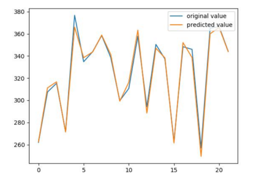
Line 71: Plot of original value is plotted using matplotlib
Line 72: Plot of machine predicted value is plotted using matplotlib
Line 73: Legend is plotted which differentiates original value and model predicted values
Line 74: Plot is shown
Please see the output
Test Score: 4.30 RMSE
Conclusion:
So in this tutorial, we have learned about keras, LSTM and why keras is suitable to run create deep neural network. We have also gone through RNN architecture and problem of vanishing gradient being solved by LSTM. We have also gone through the architecture of LSTM and how it stored the previous memory. At the end we have presented the real time example of predicting stocks prediction using Keras LSTM.
Also Read:


I found this tutorial very useful. You can also find different loss function which helps to solve different problems.
Please see this link. Hope this may help you out.
https://www.dlology.com/blog/how-to-choose-last-layer-activation-and-loss-function/
Hello, How are you. Hope you are fine. I found this link very useful.
Thanks again for sharing the link.