
![]()
In the Previous post we have seen how to start with the basics using tensorflow python. We come to some conclusion and let us draw these again. This post is all about Optimising parameters for less loss rate using optimizers tensorflow.
Code was divided into following section
Part 1: This part is used to create the graph and tensors.
Part 2: This section run the graphs or performs calculation using session object.
I suggest you please go to the previous tutorial before reading this one because it will help you a lot and *maintains* continuity in your understanding. Don’t worry, I would provide you the link for the previous tutorial as below
We will start writing the code without optimization and will see what is the loss rate. In the Second phase we will write the code which will be optimised using the gradient descent algorithm which will update the variables and decreases loss at every iteration. Don’t worry we will go step by step. Readers must stay with me and we will learn in interactive and enjoyable way.
Tensor flow Code to calculate the loss for straight line equation without any optimisation.
import tensorflow as tf
W = tf.Variable([-0.3],tf.float32)
b = tf.Variable([0.3],tf.float32)
x = tf.placeholder(tf.float32)
y = tf.placeholder(tf.float32)
linear_equation = W * x + b
init = tf.global_variables_initializer()
difference = tf.square(linear_equation-y)
loss = tf.reduce_sum(difference)
sess = tf.Session()
sess.run(init)
File_writer = tf.summary.FileWriter("path to graph",sess.graph)
print(sess.run(loss,{x:[1,2,3,4],y:[0,-1,-2,-3]}))
Explanations of the above code line wise
Line 1: Tensorflow library is imported as tf.
Line 2: Variable W stores the value which is of type float32.
Line 3: Variable b stores the value which is of type float32. Please remember that you need to initialize these variable which is implemented using tf.global_variables_initializer()
Line 4-5: Placeholder is used to hold value of x and y.
Line 6: linear equation is formed which resembles y = mx+c.
Line 7: Variables (W and b) are initialised using tf.global_variables_initializer()
Line 8: Difference between original value and predicted value is calculated where linear_equation is value predicted by model and y is the real value. Square of the difference is calculated at this step.
Line 9: Loss is calculated by summing the result came in the Line 8.
Line 10: Now we have been successful in creating the graph and now it is the time to run the session and see the real time results. Session object is created.
Line 11: Variable init which initialise W and b run here.
Line 12: Graph is written in the file which we will use to visualisation the graph using tensorboard.
Line 13: This is one of the most important line and both the values of placeholder is passed here. y is the actual value and x is the value which will be passed to linear equation and output comes in form of loss.
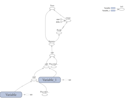
Please see the output in the tensorboard by running this line
<code>
tensorboard –logdir=path of graph file
</code>
Output of graph visualized at tensor board
Output of this code:
Tensor(“add:0”, dtype=float32)
6.859999 — This is loss
Now Please see the below code to optimise the loss using gradient descent algorithm
<code>
import tensorflow

#Trainable Parameters
W = tensorflow.Variable([0.3], dtype=tensorflow.float32)
b = tensorflow.Variable([-0.3], dtype=tensorflow.float32)
#Training Data (inputs/outputs)
x = tensorflow.placeholder(dtype=tensorflow.float32)
y = tensorflow.placeholder(dtype=tensorflow.float32)

#Linear Model
linear_equation = W * x+ b
#Linear Regression Loss Function - sum of the squares
squared_deltas = tensorflow.square(linear_equation - y)
loss = tensorflow.reduce_sum(squared_deltas)
optimizer = tensorflow.train.GradientDescentOptimizer(learning_rate=0.01)
train = optimizer.minimize(loss=loss)
#Creating a session
sess = tensorflow.Session()
writer = tensorflow.summary.FileWriter("/home/ai/PycharmProjects/tensorflow_basic/Graph1", sess.graph)
#Initializing variables
init = tensorflow.global_variables_initializer()
sess.run(init)
for i in range(500):
     (sess.run(train, feed_dict={x:[1, 2, 3, 4] , y: [0, 1, 2, 3]}))
#Print the parameters and loss
new_W, new_b, new_loss = sess.run([W, b, loss], {x: [1, 2, 3, 4], y: [0, 1, 2, 3]})
print("W : ",new_W, ", b : ",new_b, ", loss : ",new_loss)
writer.close()
sess.close()
**Some Observation in this code**: Gradient descent algorithm is used to minimize the loss. Gradient in general words means direction where maximum change takes place. THis is one of the important topic which forms base for updating weights using backpropagation method. Such change is reflected in the weight in each iteration and optimum solution is calculated. We have run the code for 500 iterations. PLEASE see the below result to see how much loss is decreased using gradient descent algorithm.
Graph can be visualised in the tensorboard by entering the following statement
<code>
tensorboard –logdir=path of graph file
Please see the path I have provided in the above code. You may change accordingly.
Let us see the new graph with optimisation
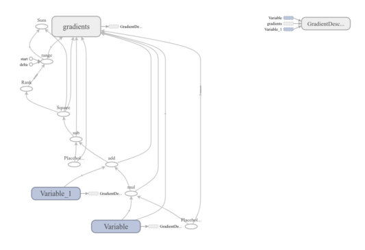
</code>
RESULTS AFTER OPTIMIZATION
(‘W : ‘, array([0.9999983], dtype=float32), ‘, b : ‘, array([-0.99999493], dtype=float32), ‘, loss : ‘, 1.762146e-11)
Conclusion:
We have concluded that using optimisation helps in finding best parameters. If you look carefully value of W = 0.3 and b= -0.3 where when optimizing algorithm run for 500 iteration it updated the value of W and b to 0.9999983 and -0.99999493 which improved loss rate from 6.859999 to 1.762146e-11. Please stay in touch with us because there is lot to come.
About AI Sangam
AI Sangam is data science solution and consulting company which focus on developing applications related to artificial intelligence, machine learning, web integration, asynchronous web sockets, docker, kubernetes, amazon ec2 instance, matlab services and tutoring. We are trying to provide you best but we need your cooperation and feedback
Follow us at
If you really like this articles please follow us at below accounts