![]()
Feed Forward Neural Network is an artificial neural network where there is no feedback from output to input. One can also treat it as a network with no cyclic connection between nodes. Let us see it in the form of diagram.
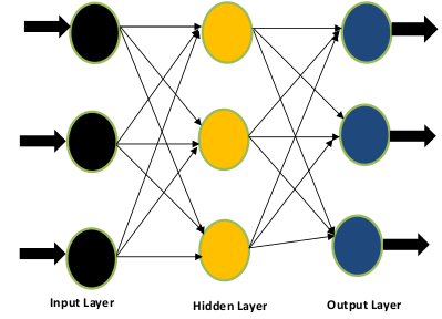
If you look carefully at Figure 1, you will notice that there are three layers (input, hidden and output layer) and flow of information is in the forward direction only. There is no backward flow and hence name feed forward network is justified.
Feedback from output to input
RNN is Recurrent Neural Network which is again a class of artificial neural network where there is feedback from output to input. One can also define it as a network where connection between nodes (these are present in the input layer, hidden layer and output layer) form a directed graph. Let us see it in form of diagram.
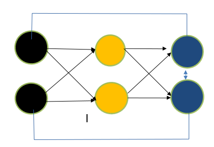
If you look at the figure 2, you will notice that structure of Feed Forward Neural Network and recurrent neural network remain same except feedback between nodes. These feedbacks, whether from output to input or self- neuron will refine the data. There is another notable difference between RNN and Feed Forward Neural Network. In RNN output of the previous state will be feeded as the input of next state (time step). This is not the case with feed forward network which deals with fixed length input and fixed length output. This makes RNN suitable for task where we need to predict the next character/word using the knowledge of previous sentences or characters/words. To know more please look at the below example.
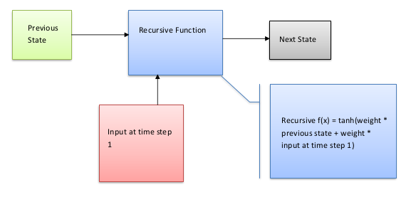
To know the flow of this Figure, let us describe this in text. RNN can memorize the input due to internal memory. It considers not only the current input but input which it receives previously. It uses the recursive function to multiple the previous input to a weight and input at time step 1 to another weight with the tanh function. Please see the below equation to understand my concept mathematically.


What is back propagation method?
This term is very important because we will discuss about vanishing gradient in the next section which depends on back-propagation. Let us understand it using the following mathematics.


Back-propagation means there is feedback from output to input which is to minimize the error between the actual output and output predicted by the model. With the help of back propagation method, we can update the weights again so that output will match the actual output. For this change in weight is calculated using the equation (3). Now the new weights are updated using the old weights and change in weight which is calculated in the equation 3.
Problem in RNN- Vanishing Gradient?????
Let us understand what is vanishing gradient as well as what is exploding gradient. Understanding of these two terms will help to understand the problem in RNN. For these we need to use equation 3 and 4. In vanishing gradient d(e)/d(w) << 1 . This will make change on weight negligible. If you calculate the new weight using the equation (4), there will negligible change in the weight which leads to vanishing gradient problem. Now let us understand what is exploding gradient problem. If d(e)/d(w) >> 1, in such case change in weight becomes quite large which makes the new weight quite large as compared to the old weight. This will leads to exploding gradient problem. There are two factors that effect the magnitude of gradient. One is weight and other is activation function. Gradients for deeper layers are calculated as the product of many gradients (activation function).
Let us explain how vanishing gradient is the problem in case of RNN.
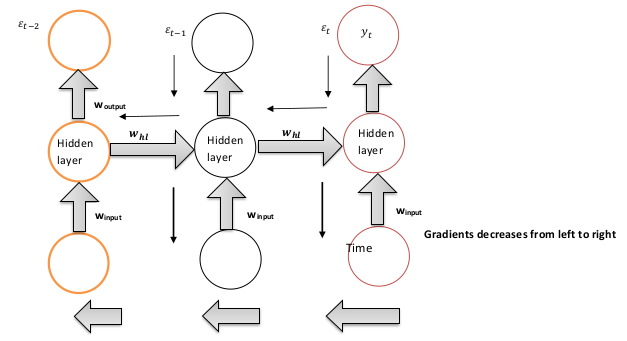
If you want to calculate the error ε It will depend to the previous states i.e. weights associated with e(t-2) and e(t-1) So when gradient (d(ε)/d(w)) is backpropagated back, all the previous weights (previous layers) needs to be updated. Problem is that when gradient is calculated it will increase towards the cost function εt but decreases while moving away from it. During training gradient associated with e(t-2) has no effect on the output (y(t)).
Understanding vanishing gradient in RNN in these key points
- Rate of change of error with respect to weight is propagated back to the time step network to minimize the cost function.
- Gradient in backward direction are calculated as product of derivatives of activation function whose magnitude is high in the hidden layers to the right and less in the hidden layers in the left.
- So when moving in the left direction gradient decreases and hence gradient is vanished.
There is another question which must come in the mind why gradient is so important with respect to above context:
Explanation to the above context is as: Gradient helps in learning. More steeper is the gradient more is the learning rate. So when the gradient degrades or becoming small learning becomes slow. This problem makes RNN not so suitable for sequential modelling when deeper context needs to be memorised and here comes the concept of LSTM (Long Short Term Memory) which we are covering in the next section.
Also Read: