Blog

Introduction

This tutorial is about creating, saving and loading the model with graph on mnist dataset (Tensorflow MNIST). You will see the tensorflow neural network on the graph. Before reading the part 5, I wish you have gone through the previous blog. If not, please spend some time in reading this.

Tensorflow control practice with live codes, graphs and sessions-Part 4 | AI Sangam

Low Level introduction of Tensorflow in a simple way – Part 3 | AI Sangam

Optimize Parameters TensorflowTutorial-Part2 | AI Sangam

Tensorflow tutorials from basic for beginners-Part 1 | AI Sangam

In this tutorial you will learn:

• Training tensorflow keras deep neural network for mnist dataset
• Graph and session for prediction phase

What you will gain after reading from this blog

• Graph and session for prediction phase
• Drawing the live graph for the prediction phase

1. Training tensorflow keras deep neural network for mnist dataset

This blog is about practical coding part so we will move directly to the code part. Special thanks to tensorflow tutorial which has helped us in creating such wonderful tutorial. First of all mnist dataset is loaded which is part of tf.keras.datasets.mnist. Please see the below code to create the module ‘tensorflow._api.v1.keras.datasets.mnist.

import tensorflow as tf
mnist = tf.keras.datasets.mnist
print(mnist)

Output of the code
module ‘tensorflow._api.v1.keras.datasets.mnist’ from ‘C:\\Python3.5\\lib\\site-packages\\tensorflow\\_api\\v1\\keras\\datasets\\mnist\\__init__.py’;

It is important to see methods available with mnist module which is created above, please run the below code

print(dir(mnist))

Output of the code
[‘__builtins__’, ‘__cached__’, ‘__doc__’, ‘__file__’, ‘__loader__’, ‘__name__’, ‘__package__’, ‘__path__’, ‘__spec__’, ‘load_data’]

As you can see in the above code, we have method load_data available with the mnist module so data is loaded using the above method as coded below

(x_train, y_train),(x_test, y_test) = mnist.load_data()

This code will load x_train, y_train, x_test and y_test. Now let us see the shape of the training and testing data as well as target using the below command

print("Please show the shape of x_train:",x_train.shape)
print("Please show the shape of x_test:",x_test.shape)
print("Please show the shape of y_train:",y_train.shape)
print("Please show the shape of y_test:",y_test.shape)

Output of the code
Please show the shape of x_train: (60000, 28, 28)
Please show the shape of x_test: (10000, 28, 28)
Please show the shape of y_train: (60000,)
Please show the shape of y_test: (10000,)

Now, let us normalize the data by dividing the x_train and x_test by 255.0. Please see the below code to get it done

x_train, x_test = x_train / 255.0, x_test / 255.0

Let us create the model using the below code

model = tf.keras.models.Sequential([
  tf.keras.layers.Flatten(input_shape=(28, 28)),
  tf.keras.layers.Dense(512, activation=tf.nn.relu),
  tf.keras.layers.Dropout(0.2),
  tf.keras.layers.Dense(10, activation=tf.nn.softmax)
])

Keras is used with tensorflow at the backend as working with tensorflow is difficult. Keras is used at the frontend which makes the task easy. Each row/sample of the training data has shape 28,28 so input shape =(28,28) is passed to the Flatten layer. Output of this layer is passed to the Dense layer with 512 neurons and activation function RELU. Deep neural network is being constructed using keras tensorflow deep learning library. To reduce the number of neurons 20 percent of them are dropped out. At the last part we pass the vectors/tensors to the last dense layer which is the softmax layer which has 10 neurons as there are 10 classes for m nist dataset (0 to 9). In this way tensorflow keras Sequential model is constructed.

Next step is to compile the model which has been created as above. To compile the model, we need  important parameters such as optimizer, loss function and metrics. Please have a look at Dlology blog to get the knowledge about which optimizer and loss function suites which type of task. Please look at the below code to get this step done.

model.compile(optimizer='adam',
              loss='sparse_categorical_crossentropy',
              metrics=['accuracy'])

Remember if you look at the mnist dataset, aim is to classify the digits from 0 to 9, hence this is treated as a category. This is the reason why loss function is chosen as sparse_categorical_crossentropy. It is a classification model and hence metrics is chosen as accuracy.

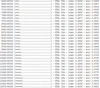
Training the model: Once you have successful in the above steps, it is vital to train the model. We have x_train and y_train from the mnist dataset. Model is trained using x_train and y_train with number of epochs. Changing the number of epochs will change the accuracy of the model. So it is important to train the model at such epoch where maximum accuracy is achieved. Please see the below code to get my point. 

model.fit(x_train, y_train, epochs=5)

Please see the screenshot to get with me at this step.

Let us save the model. Model saving will save our time because we will load the model once the model is saved and it will save our time of training the model every time to check the prediction phase. Model is saved in form of HDF5 format. If h5py is not installed in your system, please install it using the below command.

sudo pip install h5py

To save the model, please follow the below command

model.save('name.h5')

You can also save_weights of the model as well as serialize model to JSON format using the below code.

#serialize model to JSON
model_json = model.to_json()
with open("model.json", "w") as json_file:
    json_file.write(model_json)
# serialize weights to HDF5
model.save_weights("name.h5")
print("Saved model to disk")

Next step is to load the model so that we can go the prediction phase. To load the model, we need to import submodule from keras using the below code.

from keras.models import load_model
model = load_model('name.h5')

Output of the model
keras.models.Sequential object at 0x000000000AA2B208 

2. Graph and session for prediction phase

Since the model is loaded it is important to proceed to the prediction phase with graph creation using tensorflow. Please have a look at the below code how prediction phase works

x_placeholder = tf.placeholder(tf.float32, shape=(None,28,28))
y = model(x_placeholder)
x = x_test
with tf.Session() as sess:
    writer = tf.summary.FileWriter('session_tensorflow_7', sess.graph)
    sess.run(tf.global_variables_initializer())
    print("Predictions from:\ntf graph:      "+str(sess.run(y, feed_dict={x_placeholder:x})))
    print("keras predict: "+str(model.predict(x)))

Some points to remember
1.) We have taken placeholder as different values of x will be updated each with the shape of 28,28.
2.) Both the values (graph and model.predict) are printed. Along with this graph is generated. Please have a look at the below output as well as graph for this session.
3.) model.predict is used to provide the output for the testing data.
4.) Some times model is not loaded and problem of unknown initializer: GlorotUniform when loading Keras model comes so please implement the below code to rectify the problem

import keras
from keras.models import load_model
from keras.utils import CustomObjectScope
from keras.initializers import glorot_uniform

with CustomObjectScope({'GlorotUniform': glorot_uniform()}):
        model = load_model('imdb_mlp_model.h5')

Let us see the graph being plotted using the tensorflow using the above code as below

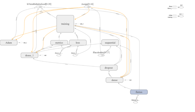
When you run the code, you will see code is using tensorflow at the backend, please visit the link C:\Users\datascience\.keras if you are using windows or /home/datascience/.keras/keras.json if you are using ubuntu. When you open such file, you will find the following content.

{
    "epsilon": 1e-07, 
    "floatx": "float32", 
    "image_data_format": "channels_last", 
    "backend": "tensorflow"
}

Please change the back-end to the tensorflow or theano. It depends on you.

What you have learned after this tutorial

In a nutshell this tutorial is about Tensorflow MNIST i.e building tensorflow neural network for mnist dataset . Proper code with both explanation as well as live graphs are shown in this blog. From my consideration, you have gained knowledge how to save the keras model as well as how to load the model. We also came across plotting the prediction phase on the graph in the tensorflow. Live sessions and practice will lead in increase interest in understanding deep learning libraries such as tensorflow. I also urge you to go through the first four tutorial on tensortflow series so that proper coordination as well as synchronization can be build. Don’t miss our video on real time face recognition.

For more such information subscribe us at our aisangam youtube channel.

Also Read:

Tensorflow control practice with live codes, graphs and sessions- Part 4 | AI Sangam